A modern optical design process relies on numerical simulations during nearly all phases of the development cycle. Be it checking the feasibility of a great new idea, optimizing the parameters of a proof-of-concept, identifying risks and tolerances in engineering or combinations of those. Perhaps you’re trying to find out if a metasurface can help you shrink down a bulky optical system, you may be worrying how tight the tolerance for placing and manufacturing flat lenses will have to be or looking to optimize your system for the highest possible efficiency.
In all these cases you will need nano-photonic modelling to compare the performance of different structures. One of the most common concerns when deciding on a simulation method is how fast the calculations are. In other words, how long will it take to produce the data needed to make sound decisions.
Fast simulations have another advantage. Because configurations are calculated faster, the parameter space that can be explored becomes larger. Expanding the parameter space in turn improves the quality of the final design.
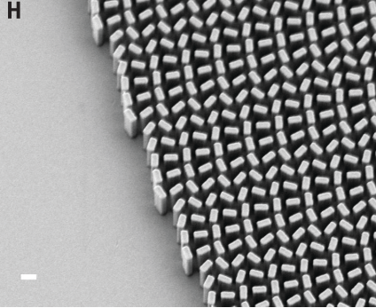
In this post we will explain the various choices that influence the calculation speed when designing meta-atoms, the sub-wavelength structures, which are the building blocks of metasurfaces. The nano-structures are designed to control the optical behaviour of the metasurface. Building a library of high performance meta-atoms with varied functionalities is essential to designing metalenses, functionalized diffraction gratings, holograms and filters. Many of the recommendations in this article apply to all kinds of optical simulations but we will focus specifically on metasurfaces.
How long do simulations take?
Let’s get straight to the point, nano-photonic calculations are time consuming. The calculation of a single configuration takes more than an hour in some cases. Sub-wavelength structures require that the complete Maxwell equations be solved in 3D (hence the term full wave simulation) to determine the electric and magnetic fields with resolutions in the nanometer range. Calculating in this level of detail is demanding in terms of processing power and memory. Volumes of more than a few tens of wavelengths (in 3 directions) are barely possible with standard PCs because the computer either runs out of memory or the simulation takes too long to be feasible.
What can be done to speed up calculations?
There are several ways to speed up the calculations or more accurately prevent the simulation time from becoming impractically long. Combining these will get the most effective simulation setup. Generally these are the options:
- Sensible choice of parameters, ranges and resolution
- Choose a performant algorithm
- Use high performance computers
The proof of the pudding: a benchmark of calculation time
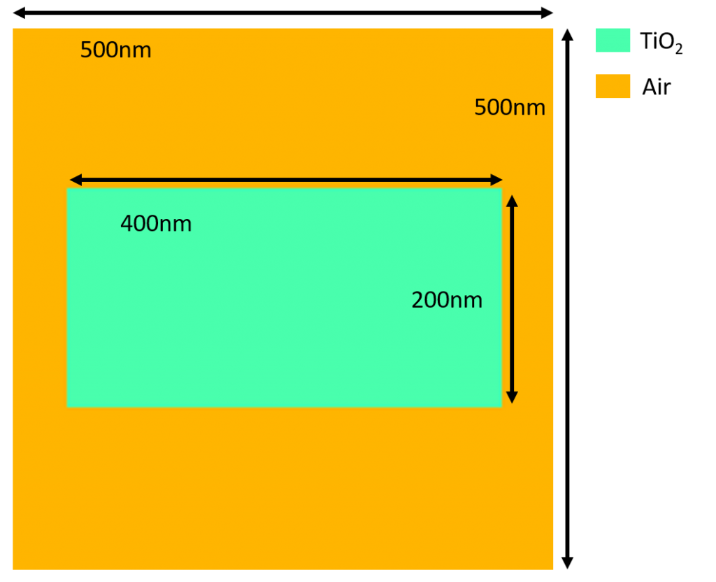
In this article we will use a well known type of meta-atom as a reference structure to compare two commonly used simulation algorithms. The reference structure uses the geometric phase (also called Pancharatnam-Berry phase) which simultaneously converts polarization and controls the phase of the transmitted light. This shape has been widely used in metalens demonstrations for example[1], [2]. When using such a structure one of the first tasks is to select the appropriate structure height which maximizes the polarization conversion efficiency. As a reference we will tune the height of the structure and analyze which accuracy settings to apply in our simulations for RCWA and FDTD simulations.
Below is a representation of the geometry and materials that were used in this example.
Choice of parameters
The first aspect is to choose the parameter space carefully. The number of calculations to run grows exponentially with the amount of parameters and the resolution with which these are varied. Consider a simple example: a brute force scan of two parameters with 20 values per parameter would take 400 calculations. Let’s assume a calculation takes 10 seconds (below you will see that this is a reasonable amount of time), that means the parameter scan will be completed in a little more than 1 hour. If we now add 2 more parameters that becomes …. 20 days.
When choosing the parameters think about the underlying physics of the structure to identify those variables that are most likely to have a major effect on the results. For example it is known from theory that rotating the rectangle will rotate the phase of the converted polarization but have a small to no effect on the conversion efficiency. We therefor keep the orientation fixed. Another good practice is to first perform a crude scan of the parameter space to identify interesting regions and later simulate the most interesting in closer detail.
Benchmark calculation speed for meta-atoms
A great deal of full wave simulation algorithms are in use today. All of those solve Maxwell’s equations and will return the same result in principle. But not all algorithms are equally fast in finding this solution. In the metasurface literature the most commonly used methods are FDTD, RCWA and FEM. These abbreviations respectively mean Finite Difference Time Domain, Rigorous Coupled Wave Analysis and Finite Element Method.
Below we compare the calculation time in relation to the accuracy settings for RCWA and FDTD two of the most popular choices. The RCWA calculations were performed using PlanOpSim’s software package, the FDTD calculations were done using the MEEP package.
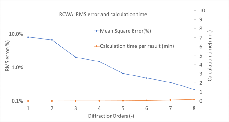
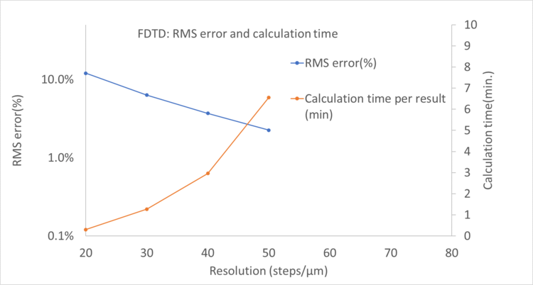
Any full wave algorithm will have to discretize the structure, this is known as discretization or meshing. The stepsize of this discretization has a large influence on the simulation time and accuracy. In practice we have to determine the smallest resolution that still returns reasonably accurate results. In FDTD this is directly controlled by how many discretization steps are taken per micrometer. In RCWA this is indirectly controlled by the number of spatial frequencies (also called diffraction orders) used to represent the geometry. Both parameters have similar effects, increasing them will increase the accuracy but also slow down the calculation.
In the plots below we show the accuracy expressed as root mean square of the error for different settings in RCWA and FDTD. Let’s say we want our simulations that have an RMS error of 1.5% or better in determining the polarization conversion efficiency. We see that we respectively need an RCWA setting of 5 diffraction orders and an FDTD resolution of 50 steps/um.
Combining the data for RCWA and FDTD above, we can look at the time per calculation compared to the RMS error. This plot is shown below. On the left side we have calculations with low error/high precision, the right side have larger errors. Naturally, when a higher precision is required the calculation will take longer.
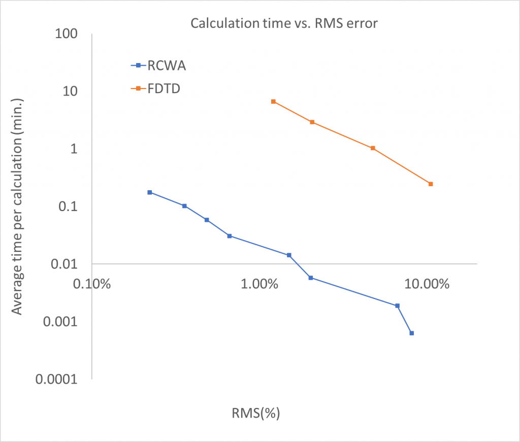
The data show that for meta-surface calculations the RCWA method returns results faster than FDTD at the same accuracy. This speed does come at a cost, RCWA is only suited for periodic structures while the FDTD method can also be applied to non-periodic structures. In practice meta-atoms are often optimized with periodic boundary conditions (this is known as the local periodic approximation). Simulating the non-periodic aspects is possible but requires very large simulation volumes with prohibitively long calculation times.
What about high performance computers
Finally the simulation time can be reduced (regardless of the method applied) by straightforward increases in computation power. Either by running on an on-premises powerful workstation or using cloud computing to flexibly scale the computation power.
To demonstrate the effect of this approach we have run the same calculation as above on the cloud using AWS and compared the calculation time to the local calculations above. On a laptop the parameter sweep was completed in 19.3 minutes. The same calculation took only 10.65 minutes on the cloud. This represents a 45% decrease in calculation time. Keeping in mind that this test was run on a modest AWS machine. Scaling further to the most powerful cloud servers would further reduce the time vs. local calculations. PlanOpSim’s software is deployed on the cloud to have this increase of computation power in reach whenever needed. A simulation running in the cloud will also not compete with other programs and will not slow down other day-to-day work.
About PlanOpSim
PlanOpSim develops dedicated simulation software for the design of metasurfaces, metalenses and other planar optical components. Contact us with any questions or to evaluate the software.
References
[1] M. Khorasaninejad, W. T. Chen, R. C. Devlin, J. Oh, A. Y. Zhu, and F. Capasso, “Metalenses at visible wavelengths: Diffraction-limited focusing and subwavelength resolution imaging,” Science (80-. )., vol. 352, no. 6290, pp. 1190–1194, 2016.
[2] D. Lin et al., “Polarization-independent metasurface lens employing the Pancharatnam-Berry phase,” Opt. Express, vol. 26, no. 19, p. 24835, 2018.